PID is the proportional calculus adjustment, you can refer to the automatic control course in detail! Positive action and negative reaction In the temperature control, it is heating when positive action, and reaction control is refrigeration control. Introduction to PID Control The current level of industrial automation has become an important indicator of the level of modernization in all walks of life. At the same time, the development of control theory also experienced three stages: classical control theory, modern control theory, and intelligent control theory. Typical examples of intelligent controls are fuzzy automatic washing machines. Automatic control systems can be divided into open-loop control systems and closed-loop control systems. A control system includes controllers, sensors, transmitters, actuators, and input and output interfaces. The output of the controller is added to the controlled system through the output interface and actuator, and the controlled volume of the control system is sent to the controller via the input interface via sensors and transmitters. Different control systems have different sensors, transmitters, and actuators. For example, pressure control systems use pressure sensors. The sensor of the electric heating control system is a temperature sensor. At present, there are many PID controllers and their controllers or intelligent PID controllers (instruments). The products have been widely used in engineering practice. There are various PID controller products. All major companies have developed PIDs. Self-tuning parameter intelligent regulator (intelligentregulator), which PID controller parameters automatically adjust through intelligent adjustment or self-correction, adaptive algorithm to achieve. There are pressure, temperature, flow, level controllers that use PID control, programmable controllers (PLC) that can implement PID control functions, and PC systems that can implement PID control. 1, open-loop control system An open-loop control system means that the output (controlled amount) of the controlled object has no effect on the output of the controller. In such a control system, it does not rely on sending back the controlled quantity to form any closed loop. A closed-loop control system is characterized in that the output of the system controlled object (the controlled variable) is sent back to affect the output of the controller, forming one or more closed loops. The closed-loop control system has positive feedback and negative feedback. If the feedback signal is opposite to the system setpoint signal, it is called negative feedback (NegativeFeedback). If the polarity is the same, it is called positive feedback. Generally, the closed-loop control system uses negative feedback. Also known as negative feedback control system. There are many examples of closed-loop control systems. For example, a human being is a closed-loop control system with negative feedback. The eye is a sensor and acts as a feedback. The human body system can make various correct actions through continuous correction. Without eyes, there is no feedback loop and it becomes an open-loop control system. In another example, when a genuine fully automatic washing machine has the ability to continuously check whether the laundry is washed and can automatically cut off the power after washing, it is a closed-loop control system. The step response is the output of the system when a step function is added to the system. Steady-state error refers to the difference between the expected output and the actual output of the system after the response of the system has entered the steady state. The performance of the control system can be described in terms of stability, accuracy, and speed. Stability refers to the stability of the system. A system must be able to work properly. It must be stable first, and it should be convergent from the point of view of step response. It refers to the accuracy and control accuracy of the control system and is usually stabilized. Steady-state error describes the difference between the steady-state value of the system output and the expected value. Fast refers to the rapidity of the response of the control system and is usually described quantitatively by the rise time. In engineering practice, the most widely used regulator control law is proportional, integral, differential control, referred to as PID control, also known as PID regulation. The PID controller has been in existence for nearly 70 years. With its simple structure, good stability, reliable work, and easy adjustment, it has become one of the main technologies for industrial control. When the structure and parameters of the controlled object cannot be fully grasped or the precise mathematical model cannot be obtained, when the other techniques of the control theory are difficult to adopt, the structure and parameters of the system controller must be determined by experience and on-site debugging. PID control technology is the most convenient. That is, when we do not fully understand a system and controlled object, or cannot obtain system parameters through effective measurement methods, it is most suitable to use PID control technology. PID control, actually there are PI and PD control. PID controller is based on the system error, using the proportional, integral, differential calculation of the control of the amount of control. Proportional (P) Control Proportional control is the simplest type of control. The output of the controller is proportional to the input error signal. When there is only proportional control, there is a Steady-state error in the system output. Integral (I) Control In integral control, the output of the controller is proportional to the integral of the input error signal. For an automatic control system, if there is a steady-state error after entering the steady state, the control system is said to have a steady-state error or a system with a difference (System with Steady-state Error). In order to eliminate the steady-state error, an "integral term" must be introduced in the controller. Integral term pair error depends on the time of the integral, as time increases, the integral term will increase. In this way, even if the error is small, the integral term will increase with time. It will push the increase of the output of the controller to further reduce the steady-state error until it reaches zero. Therefore, the proportional + integral (PI) controller can make the system have no steady state error after entering the steady state. Derivative (D) control In derivative control, the output of the controller is proportional to the derivative of the input error signal (ie, the rate of change of the error). The automatic control system may oscillate or even lose stability in overcoming the error adjustment process. The reason is that due to the presence of larger inertial components (links) or delay components, it has the effect of suppressing errors, and the change always lags behind the change of error. The solution is to "lead" the change in the effect of the suppression error, ie when the error is close to zero, the effect of the suppression error should be zero. This means that introducing only the “proportional†term in the controller is often not enough. The proportional term only acts as the magnitude of the amplification error, and what is currently needed to increase is the “differential termâ€, which can predict the trend of error variation. In this way, a controller with proportional + differential can make the control action of the suppression error equal to zero or even negative in advance, thereby avoiding a serious overshoot of the controlled volume. Therefore, for the controlled object with large inertia or lag, the proportional plus derivative (PD) controller can improve the dynamic characteristics of the system during the adjustment process. The parameter setting of the PID controller is the core content of the control system design. It is based on the characteristics of the controlled process to determine the size of the PID controller's proportional coefficient, integration time and derivative time. There are many ways to set PID controller parameters. There are two general categories: The first is the theoretical calculation method. It is mainly based on the system's mathematical model, through the theoretical calculation to determine the controller parameters. The calculation data obtained by this method may not be directly used, but must also be adjusted and modified through actual engineering. The second is the engineering setting method. It mainly relies on engineering experience, directly in the test of the control system, and the method is simple, easy to master, widely used in the actual project. The engineering tuning methods for PID controller parameters include critical ratio method, response curve method and attenuation method. Each of the three methods has its own characteristics. Its common point is to pass the test, and then adjust the controller parameters according to the engineering experience formula. However, no matter which method is adopted, the controller parameters need to be adjusted and improved in the actual operation. The critical ratio method is now generally used. Use this method to set the PID controller parameters as follows: (1) First select a short enough sampling period for the system to work; (2) Add only the proportional control link until the system has a critical oscillation of the step response to the input, and note the proportional amplification factor and the critical oscillation period at this time; (3) The parameters of the PID controller are calculated by the formula under a certain degree of control. PID parameter setting: It is familiar with experience and process, reference measurement value tracking and set value curve, so as to adjust the size of P\I\D. PID controller parameter engineering setting, PID parameter empirical data of various regulation systems The following can refer to: Temperature T: P=20~60%, T=180~600s, D=3-180s Pressure P:P=30~70 %, T=24~180s, liquid level L: P=20~80%, T=60~300s, flow rate L: P=40~100%, T=6~60s. Commonly used formulas in the book: parameter setting to find the best, from the smallest to the largest, the first is the proportion after the first, and then the differential plus the curve is very frequent oscillation, the proportional dial to enlarge the curve floating around the big bay, the proportional dial to the small pull curve Deviation from the slow response, the integration time to the downward curve of the long cycle of fluctuations, the integration time and then increase the long curve oscillation frequency, the first differential down to large fluctuations in slow fluctuations. Differential time should lengthen the two waves of the ideal curve, before the high and low 4 to 1 to see two more analysis, the quality of the adjustment will not be low Here is an empirical method. This method is essentially a trial and error method. It is an effective method that has been summarized in the production practice and has been widely used in the field. The basic procedure of this method is to first determine a set of regulator parameters based on operating experience, and put the system into closed-loop operation, then artificially add step disturbances (such as changing the regulator's given value), observe the adjusted or adjusted The output of the step response curve. If it is considered that the control quality is unsatisfactory, the controller parameters are changed according to the influence of each setting parameter on the control process. This trial and error until satisfied. The empirical method is simple and reliable, but it requires certain on-site operational experience, and it is subjective and subjective one-sided. When using a PID regulator, there are a number of tuning parameters, and the number of trial and error times increases, and it is not easy to obtain the optimal tuning parameters. The following takes the PID regulator as an example to specify the steps for setting the empirical method: (2) Take the proportional coefficient S1 as the current value multiplied by 0.83, increase the integral coefficient S0 from small to large, and let the disturbance signal make step changes, until a satisfactory control process is obtained. (3) The integral coefficient S0 remains unchanged, change the proportional coefficient S1, observe whether the control process has improved, if there is improvement, continue to adjust until satisfactory. Otherwise, increase the original proportional coefficient S1 and adjust the integral coefficient S0 to improve the control process. Repeat this trial and error until you find a satisfactory scale factor S1 and the integral factor S0. (4) Introduce the appropriate actual differential coefficient k and the actual derivative time TD. At this time, the proportional coefficient S1 and the integral coefficient S0 can be appropriately increased. As with the previous steps, the setting of the differential time also needs to be adjusted repeatedly until the control process is satisfied. Note: The PID regulator used in the simulation system is different from the traditional industrial PID regulator. Each parameter is isolated from each other and does not affect each other. Therefore, it is very convenient to observe the regulation rules with it. PID parameters are determined based on the inertia of the control object. Large inertia, such as: large drying room temperature control, generally P can be more than 10, I = 3-10, D = 1 or so. Small inertia such as: A small motor with a pump for pressure closed-loop control, generally only PI control. P = 1-10, I = 0.1-1, D = 0, these should be corrected during on-site commissioning. I provide an incremental PID for your reference. ΔU(k)=Ae(k)-Be(k-1)+Ce(k-2) A=Kp(1+T/Ti+Td/T) B =Kp(1+2Td/T) C=KpTd/TT Sampling Period Td Differentiation Time Ti Integral Time The above algorithm can be used to construct its own PID algorithm. U(K)=U
This product response time is shorter than resistive tonch screen's with a good touch.It is widely used to Phone,Tablet,E-book,gaming device by hands holding,Touch Monitor,GPS,All-In-One and so on.GreenTouch projected capacitive touch technology is with fast and sensitive response, the design with frame (without frame is optional) makes it looks professional and generous. The model is designed for high-intensity and high-frequency business environments.
Product show:
Capacitive Touch Screen Panel,Android Touch Screen,Portable Touch Screen,Pcap Touch Screen,POS Terminal Touch Screen,Mini Capacitive Touch Screen ShenZhen GreenTouch Technology Co.,Ltd , https://www.bbstouch.com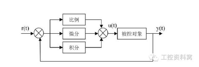
(1) Let the regulator parameter integral coefficient S0 = 0, the actual differential coefficient k = 0, the control system put into closed-loop operation, change the proportional coefficient S1 from small to large, let the disturbance signal make a step change, observe the control process, until obtaining satisfactory control Process. 


